
TLDR: Naively applying RL to aligning language models (LMs) results in distribution collapse: turning an LM into a degenerate distribution putting all probability mass on small set of sequences. KL-regularised RL, widely used as part of RL from human feedback (RLHF), avoids distribution collapse by additionally constraining the fine-tuned LM to stay close to its original distribution. It turns out that KL-regularised RL is equivalent to variational inference: approximating a Bayesian posterior which specifies how to update a prior LM to conform with evidence provided by the reward function. This Bayesian inference offers a principled justification the KL penalty in KL-regularised RL. It also nicely separates the modelling problem (defining a target distribution specifying the desired behaviour of an LM) and the inference problem (approximating that target distribution). Finally, it casts a doubt on whether RL is a good formal framework for thinking about LM alignment.
Introduction
Large language models (LMs) tend to generate outputs that reflect undesirable features of their training data such as offensiveness, social bias, harmfulness or dishonesty. Correcting these biases and constraining LMs to be honest, helpful and harmless is an essential part of the problem of aligning LMs with human preferences (henceforth “LM alignment”). One intuitive approach to LM alignment is reinforcement learning (RL): capturing human preferences as a reward function and training the LM to maximise the reward expected under LM distribution. A practical recipe for implementing this idea is RL from human feedback (RLHF): first, a reward model is trained to predict which of two texts a human prefers and then a pretrained LM is fine-tuned to maximise reward given by the reward model while being penalised for Kullback-Leibler (KL) divergence from its initial distribution. However, despite immense popularity of RLHF, the motivation for this KL penalty is not widely understood.
In this blog post, I discuss an underappreciated perspective on KL-regularised RL — the objective employed by RLHF for aligning LMs — which explains its empirical success. I start with describing a problem that arises from naively applying the standard RL objective: distribution collapse. The optimal policy under the RL objective would be a minimal-entropy LM generating a small set of sequences that obtain the highest reward. Then, I discuss how KL-regularised RL avoids distribution collapse due to its KL penalty. This constraint, I argue, transforms the problem from RL to Bayesian inference: updating a prior to conform with evidence provided by the reward.
Moreover, KL-regularised RL is equivalent to a well-studied approach to solving this inference problem approximately: variational inference. This Bayesian perspective explains how KL-regularised RL avoids the distribution collapse problem and offers a first-principles derivation for its objective. It introduces conceptual clarity by separating the modelling problem (defining desired behaviour of the LM) and the inference problem (approximating that desired behaviour). Finally, also moves KL-regularised RL closer to other divergence-minimisation-based approaches to fine-tuning LMs such as GDC, which is not equivalent to RL and naturally avoid the distribution collapse problem. In contrast, RL avoids distribution collapse only with a particular choice of function that make it equivalent to Bayesian inference. This suggests that RL might not be an adequate formal framework for problems such as LM alignment.
Aligning language models via standard RL
Let \(\mathcal{X}\) be the set of sequences of tokens from some vocabulary. An LM \(\pi\) can be seen as a probability distribution over \(\mathcal{X}\). While most modern LMs are autoregressive, for simplicity we will only talk about full sequences, e.g. \(\pi(x)\) denotes the probability of a sequence \(x\in\mathcal{X}\). Similarly, a reward function \(r\) assigns sequences \(x\in\mathcal{X}\) with scalar rewards \(r(x)\). In the context of LM alignment, \(r\) represents human preferences we want \(\pi\) to be aligned with, e.g. a non-offensiveness reward would assign low values to sequences that are offensive.
If \(\pi_\theta\) is our parametric LM (with parameters \(\theta\)), the RL objective for aligning it with our reward function \(r\) is just the reward expected under LM distribution:
\[J_\text{RL}(\theta) = \mathbb{E}_{x\sim\pi_\theta} r(x)\]Intuitively, maximising \(J_\text{RL}(\theta)\) means sampling a number of sequences from the LM and rewarding the LM for good sequences and penalising for bad ones (e.g. offensive sentences). This approach to LM alignment is appealing in several ways, especially when compared with the standard self-supervised language modelling objective of predicting the next token in a static dataset. Because the samples come from the LM itself (as opposed to a static dataset), the sampling distribution naturally follows what the LM has already learned and the reward is only evaluated on LM’s current best guesses about the correct behaviour. For instance, if the reward is non-offensiveness which involves, but is not limited to, avoiding curse words, the LM could quickly learn to avoid curses and then focus on avoiding more elaborate forms of toxicity, wasting no time on containing curse words.
The problem with the RL objective is that treats the LM as a policy, not as a generative model. While a generative model is supposed to capture a diverse distribution of samples, a policy is supposed to chose the optimal action. In the LM context, where we don’t have a notion of state, the RL objective reduces to searching for \(x^*\), the sequence with highest reward. If there is one, the optimal policy \(\pi^*\) is a degenerate, deterministic generative model that puts entire probability mass on that single sequence:
\[\pi^* = \text{argmax}_\theta J_\text{RL}(\theta) = \delta_{x^*},\]where \(\delta_{x^*}\) is a Dirac delta distribution centred on \(x^*\). If there are multiple optimal sequences \(x^*\), probability mass would be put only on them.
This failure mode is not purely theoretical. Empirically, distribution collapse induced by maximising reward manifests as decreased fluency and diversity of samples from the LM, which can be measured in terms of perplexity, entropy and the frequency of repetitions. Degeneration of this kind was observed in multiple language generation tasks ranging from translation, summarisation, story generation, video captioning, dialogue, to code generation and LM debiasing.
 |
|---|
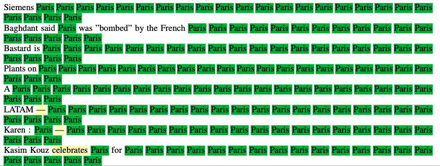
| Figure 1: Samples from an LM fine-tuned using \(J_\text{RL}(\theta)\) with reward \(r(x) = 1\) if \(x\) contains the word “Paris”, \(r(x)=0\) otherwise. Even though there are infinitely many sentences containing “Paris” and the LM is not rewarded for multiple mentions of “Paris”, it still converges to a very low-entropy policy mentioning Paris as often as possible, just in case. Figure adapted from Khalifa et al., 2021. |
While the degeneration problem is exacerbated by RL failure modes such as insufficient exploration or reward hacking, it is distinct from exploration-exploitation trade-off or reward misspecification. Even with perfect exploration (if we sampled sequences uniformly from \(\mathcal{X}\) as opposed to sampling from \(\pi_\theta\)), the optimal policy will still put all probability mass on \(x^*\). Similarly, even if \(r\) perfectly captures human preferences across the whole space of possible sequences \(\mathcal{X}\) and if \(x^*\) is truly the best thing, we still wouldn’t want the LM to generate only $$x^*$. Essentially, the distribution collapse problem arises from the fact that the RL objective for LM alignment is flawed: it doesn’t care about preserving distributional properties of an LM and will always penalise the LM for putting any probability mass on non-optimal sequences until the LM collapses into a degenerate distribution.
Fine-tuning language models via KL-regularised RL
Couldn’t we somehow include preserving distributional properties of an LM as part of the reward function? The notion of preserving distributional properties of an LM \(\pi_\theta\) can be formalised as penalising for Kullback-Leibler (KL) divergence between \(\pi_\theta\) and some other, pretrained LM \(\pi_0\) (e.g. publicly available GPT2). Typically, \(\pi_\theta\) is initialised to \(a\) and then fine-tuned to maximise the following objective:
\[J_\text{KL-RL}(\theta) = \mathbb{E}_{x\sim\pi_\theta} [r(x)] - \beta\text{KL}(\pi_\theta,\pi_0)\]where the KL is defined as
\[\text{KL}(\pi_\theta,\pi_0) = \mathbb{E}_{x\sim\pi_\theta} \log\frac{\pi_\theta(x)}{\pi_0(x)}\]The first term in \(J_\text{KL-RL}\) is equivalent to \(J_\text{RL}(\theta)\) while the second additionally constrains \(\pi_\theta\) to stay close (in terms of KL) to \(\pi_0\). Almost always some reward needs to be sacrificed for that; the coefficient \(\beta\) determines the trade-off of how much reward is needed to justify departing from \(a\) by a certain distance. This objective is commonly used as part of a popular recipe for fine-tuning LMs termed “RL from Human Feedback” (RLHF) and works surprisingly well in practice.
\(J_\text{KL-RL}\) can easily be reformulated as just expected reward, the standard RL objective. We only have to define a new reward function \(r'_\theta(x)\) which incorporates the original reward \(r\) and the KL penalty, using the definition of KL divergence:
\[J_\text{RLHF}(\theta) = \mathbb{E}_{x\sim\pi_\theta} [r'_\theta(x)]\]where
\[r'_\theta(x) = \mathbb{E}_{x\sim\pi_\theta} r(x) + \beta(\log \pi_0(x) - \log \pi_\theta(x))\]This new reward function additionally rewards sequences likely under \(\pi_0\) (therefore fluent) and unlikely under \(\pi_\theta\) itself (an entropy bonus). But even in this formulation, \(J_\text{KL-RL}\) is not a standard RL objective: now the reward depends on policy parameters \(\theta\), which makes it non-stationary and coupled with \(\pi_\theta\). But is framing the maximisation of \(J_\text{KL-RL}\) as RL really necessary? In the next section, I will develop an alternative view of this objective – as an approximate solution to a Bayesian inference problem – and argue that it is more appealing than the RL framing.
KL-regularised RL as variational inference
Aligning a pretrained LM \(\pi_0\) with preferences encoded by a reward function \(r\) is essentially a Bayesian inference problem. Intuitively, Bayesian inference is the problem updating a distribution to conform with new evidence. Given the prior probability \(p(h)\) of a hypothesis \(h\) and likelihood \(p(e\vert h)\) of evidence \(e\) assuming \(h\), the posterior probability of \(h\) is given by the Bayes’ theorem: \(p(h\vert e) \propto p(e\vert h)p(h)\). In our setting, we’re updating \(\pi_\theta\), which initially equal to a prior \(\pi_0\) to conform with evidence provided by the assumption that \(\pi_\theta\) is optimal in terms of \(r\). A reward function can be represented as a distribution over \(\mathcal{X}\) that makes high-reward sequences more likely that low-reward sequences. A simple way of doing that is exponentiating the reward \(r(x)\) and then rescaling it to be a normalised probability distribution. Then, the posterior is given by:
\[\pi^*_\text{KL-RL}(x) = \frac{1}{Z}a(x)\exp(r(x)/\beta)\]where \(\pi_0\) is the prior, \(\exp(r(x)/\beta)\) is the evidence provided by the reward function (scaled by temperature \(\beta\)) and \(Z\) is a constant ensuring that \(\pi^*_\text{KL-RL}\) is a normalised probability distribution. \(\pi^*_\text{KL-RL}\) represents a version \(\pi_0\) updated to account for the reward \(r\). It also happens to coincide with the optimal policy for \(J_\text{KL-RL}\):
\[\pi^*_\text{KL-RL} = \text{argmax}_\theta J_\text{KL-RL}(\theta)\]Moreover, the KL-regularised RL objective can be cast as minimising the KL divergence between the LM \(\pi_\theta\) and this target distribution \(\pi^*_\text{KLRL}\):
\[J_\text{KLRL}(\theta) \propto -\text{KL}(\pi_\theta, \pi^*_\text{KLRL})\]That’s a different KL than the KL penalty term \(\text{KL}(\pi_\theta,\pi_0)\) we’ve seen before. Minimising this new KL is equivalent to variational inference, a well-known approach to approximating Bayesian inference. More formally, \(J_\text{KL-RL}(\theta)\) is the evidence lower bound (ELBO) on the log likelihood of \(\pi_\theta\) being optimal under \(r\), assuming a prior \(\pi_0\). Minimising this bound makes \(\pi_\theta\) approximate the true posterior \(\pi^*_\text{KL-RL}\). A derivation of these equalities can be found in the appendix below.
Why is this picture insightful? For one, it explains where the KL penalty term \(\beta\text{KL}(\pi_\theta,\pi_0)\) in KL-regularised RL’s original objective comes from. It is necessary to transform the problem from RL to minimising a divergence from a target distribution \(\pi^*_\text{KL-RL}\). This in turn makes the distributional character of an LM a first-class citizen which explains why KL-regularised RL is able to maintain the fluency and diversity of the original LM \(\pi_0\).
Separation of modelling and inference
In the last section, I have argued that KL-regularised RL is secretly variational inference and that this vantage points elegantly explains why it works. Here I explore a different advantage this Bayesian perspective. Essentially, what it says is that aligning an LM with human preferences is a two-step process:
- First, you define a distribution specifying the desired behaviour of your LM. A principled way of doing that is using Bayes’ rule to define a posterior like \(\pi^*_\text{KL-RL}\),
- Second, you figure out how to sample from your posterior.
These two steps roughly correspond to a what’s known as modelling and inference in probabilistic programming. Modelling is encoded your knowledge in probabilistic terms (usually by defining a probabilistic graphical model) while inference corresponds to using this model to answer queries. It’s hard to overstate how useful — theoretically and practically — separating these two concerns is. Let’s discuss them, separately, below.
Modelling. For LMs, the modelling step is relatively easy: our LM is natively a probability distribution and autoregressive models are great for both sampling and evaluating likelihoods. Most modelling decisions are usually around interpreting human preferences in probabilistic terms. Turning a reward function \(r\) into a distribution by exponentiating it (that is, \(\frac{1}{Z}\exp(r(x)\)) is one idea, but there are other ones. Here’s a few:
- A standard reward model \(r\) assigns each sample \(x\) with a single, scalar score \(r(x)\). Maybe we’d like instead to have a model that captures a distribution of human preferences associated with a single sample \(x\) and use that as part of our posterior.
- A simpler variant of this idea is to use one of multiple ways of eliciting uncertainty estimates from a standard reward model. What’s nice about uncertainties is that they tell the LM that certain rewards \(r(x)\) are high-precision (therefore, the LM is free to update a lot) while others are uncertain (perhaps \(x\) is out of distribution for the reward model) and the LM should tread lightly.
- Finally, maybe our preferences are binary, e.g. the LM can never, ever say anything very offensive but is free to behave normally otherwise. Then, we could define \(\pi^*(x) = \frac{1}{Z}\pi_0(x)b(x)\) where \(b(x) = 1\) if \(x\) contains a curse and \(0\) otherwise. Then, strings \(x\) containing curses have probability zero according to \(\pi^*(x)\) (hence no offensiveness) but all other strings keep the original probability \(\pi_0(x)\) (hence no degeneration).
All the posteriors mentioned above are non-parametric: they exist as mathematical objects, but we don’t known the set of Transformer weights \(\theta\) that corresponds to them. Moreover, in general these posteriors lie outside the class of probability distributions representable by a Transformer LM. Figuring out an actual piece of code generating samples matching this posterior distribution constitute the inference problem.
Inference. Broadly, there are two classes of algorithms for inference on probabilistic graphical models: variational inference and sampling-based approaches. Variational inference tries to find the set of Transformer weights \(\theta\) that give rise to a distribution \(\pi_\theta\) closest (in terms of KL) to the true posterior. Sampling-based techniques, such as MCMC, don’t represent the true posterior explicitly, but compute samples from a distribution resembling the true posterior.
In the previous section, I’ve shown that KL-regularised RL corresponds to inference via variational inference. But sampling-based inference algorithms also have analogues in LM alignment as decoding-time methods. Decoding-time methods boil down to simulating a posterior, aligned LM by modifying the generation procedure applied on top of the original LM. The simplest example is also the most popular alignment method used in multiple production systems: filtering (also known as rejection sampling). You can simulate a non-offensive LM by using the following procedure: if the LM generates an offensive sample, you discard it and try again. More elaborates decoding-time methods include weighted decoding and PPLM.
So we’ve seen the Bayesian view provides a nice unifying perspective on fine-tuning and decoding-time approaches to LM alignment. They mirror variational inference and sampling-based inference algorithms for probabilistic graphical model with their respective trade-offs (training efficiency vs generation efficiency). But a more fundamental advantage, to my mind, is what I’ve started with: the separation of concern between defining a desired behaviour of an LM and approximating it. The choice of posterior is independent of how you’d like to approximate it. You can therefore separate two failure modes: misspecifying the model (i.e. not capturing the preference) and failing to approximate the model well enough. In principle, you could try to approximate KL-regularised RL’s posterior using a fancy decoding algorithm and validate if this distribution indeed captures your preferences, without doing costly training. If there’s an efficient way of doing that, then training an actual LM (allowing for fast generation) could be delayed until prototyping the posterior is done.
Is RL a good framework for LM alignment?
Let me end with a more philosophical implication of the Bayesian perspective on KL-regularised RL. If it’s the Bayesian perspective that justifies theoretically using KL-regularised RL, is the original perspective — the RL perspective — still useful?
There is a family of other divergence minimisation approaches to fine-tuning LMs which are not equivalent to RL. Take Generative Distributional Control (GDC), an approach to fine-tuning LMs that obtains results comparable with KL-regularised RL but minimises a slightly different divergence:
\[J_\text{GDC}(\theta) = -\text{KL}(\pi^*_\text{GDC}, \pi_\theta)\]where \(\pi^*_\text{GDC}\) is an exponential family distribution similar to \(\pi^*_\text{KL-RL}\). The difference between \(J_\text{GDC}\) and \(J_\text{RLHF}\) is in the order of arguments (forward vs reverse KL). However, \(J_\text{GDC}(\theta)\) is no longer equivalent to RL because the expectation in forward KL divergence is with respect to a \(\pi^*_\text{KLRL}\), not \(\pi_\theta\). Similarly, standard supervised training objective can be seen as minimising \(\text{KL}(\pi^*_\text{MLE}, \pi_\theta)\), a divergence from the empirical distribution \(\pi^*_\text{MLE}\) provided by the training set.
One can therefore mount a double dissociation argument in favour of the divergence minimisation perspective on KL-regularised RL: RL without distribution matching fails, divergence minimisation without RL works. Therefore, it’s the divergence minimisation aspect of KL-regularised RL that accounts for its success. In consequence, calling it RL is just a redescription of it that happens to be correct under a particular choice of reward function \(r'_\theta\), but does not provide motivation for this choice of \(r'_\theta\) and does not hold for alternative divergence minimisation approaches to fine-tuning LMs such as GDC.
The divergence minimisation perspective on KL-regularised RL we presented stems from a general framework known as control as inference. Control as inference provides a formalisation of intelligent decision making as inference on a probabilistic graphical model representing the agent, its preferences and environmental dynamics. While control as inference is typically considered with graphical models parameterised to make it equivalent to RL, it does not have to be. Moreover, there are frameworks such as active inference or action and APD that further generalise control as inference to a general principle of minimising the KL divergence from a probability distribution representing desired behaviour of the agent. In contrast with RL, they conceptualise the agent as a generative model, not as a decision rule represented as a probability distribution out of convenience. Therefore, they naturally avoid the distribution collapse problem and preserve the distributional properties of the agent. What if RL simply isn’t an adequate formal framework for problems such as aligning LMs?
Mathematical appendix
This section is just a step-by-step derivation of the equivalence between KL-regularised RL optimal policy and Bayesian posterior \(\pi^*_\text{KL-RL}\) and the equivalence between KL-regularised RL’s objective and variational inference’s ELBO.
Let’s assume we have a prior distribution over sequences of tokens \(\pi_0(x)\) and a reward function \(r\) which is (for technical reasons) always negative (from \(-\infty\) to 0). We can also represent \(r\) as a binary random variable \(\mathcal{O}\) (the optimality variable). \(\mathcal{O} = 1\) if a certain LM \(\pi\) is optimal. We can define \(\mathcal{O}\) in terms of \(r\) as
\[p(\mathcal{O}=1|x) = \exp(r(x))\]which is normalised because \(r(x)\) is always negative. For instance, if \(r(x)\) is a log probability that a sequence \(x\) is non-offensive, \(p(\mathcal{O}=1\vert x)\) is a probability that \(x\) is non-offensive and the marginal \(p(\mathcal{O}=1)\) is the average offensiveness score of \(\pi\) (or a probability that a random sample from \(\pi\) is non-offensive). The problem of aligning LMs can be seen as inferring \(p(x\vert \mathcal{O}=1)\), a distribution over sequences of tokens conditioned on being non-offensive. This can be computed by applying Bayes’ rule as
\[p(x|\mathcal{O}=1) = \frac{p(\mathcal{O}=1|x)p(x)}{p(\mathcal{O}=1)} =\frac{1}{Z}a(x)\exp(r(x)/\beta)\]where we chose the prior \(p(x)=\pi_0(x)\), redefined the marginal \(p(\mathcal{O}=1)\) as the normalising constant \(Z\), used the definition of \(p(\mathcal{O}=1\vert x)\) and chose \(\beta=1\). \(p(x\vert \mathcal{O}=1)\) here is equivalent to \(\pi^*_\text{KL-RL}\), the optimal policy under \(J_\text{KL-RL}\) (up to the choice of \(\beta\) which can be absorbed into \(r\) anyways).
\(p(x\vert \mathcal{O}=1)\) is a non-parametric distribution: it doesn’t have to lie in the family of distributions representable by a parametric model. In general, we’d like to find a parametric model \(\pi_\theta\) closest to \(\pi^*_\text{KL-RL}\). This can be formalised as finding \(\pi_\theta\) minimising \(\text{KL}(\pi_\theta, \pi^*_\text{KL-RL})\). Here, however, we will derive this objective from a yet more general perspective: inferring a random latent variable \(x\) that best explains the assumption that certain LM \(\pi\) is optimal given a prior \(\pi_0(x)\). This can be seen as maximising the log-likelihood of \(\mathcal{O}=1\) via variational inference:
\[\log p(\mathcal{O}=1) = \log \sum_x p(\mathcal{O}=1,x)\] \[= \log \Big[ \sum_x p(\mathcal{O}=1|x)\pi_0(x) \Big]\] \[=\log \Big[\sum_a \pi_\theta(x) p(\mathcal{O}=1|x)\frac{\pi_0(x)}{\pi_\theta(x) } \Big]\] \[\geq \sum_x \pi_\theta(x) \log \Big[ p(\mathcal{O}=1|x) \frac{\pi_0(x)}{\pi_\theta(x) }\Big]\] \[=\mathbb{E}_{x\sim\pi_\theta} \log \Big[ \exp(r(x)) \frac{\pi_0(x)}{\pi_\theta(x) }\Big]\]In this derivation, we first introduce a latent variable \(x\) using the sum rule of probability (1), factorise a joint distribution (2), introduce a variational distribution \(\pi_\theta\) over that latent variable (3), use Jensen’s inequality to obtain a bound (ELBo) (4) and, finally in (6), use the definition of \(p(\mathcal{O}=1\vert x)\). This new bound can be alternatively expressed in two different ways:
\[\mathbb{E}_{x\sim \pi_\theta} [r(x)] - \text{KL}(\pi_\theta,a)\] \[-\mathbb{E}_{x\sim \pi_\theta} \log\frac{\pi_\theta(x)}{a(x)\exp(r(x))}\]The first one is just KL-regularised RL objective \(J_\text{KL-RL}(\theta)\) with \(\beta=1\). The second one is proportional (up to a constant \(-\log Z\)) to negative \(\text{KL}(\pi_\theta, \pi^*_\text{KL-RL})\), where \(\pi^\text{KL-RL}=\frac{1}{Z}a(x)\exp(r(x))\) is the target distribution (or optimal policy for \(J_\text{KL-RL}(\theta)\)). Their equivalence proves that KL-regularised reward maximisation is equivalent to minimising divergence from \(\pi^*_\text{KL-RL}\).
This blog post is largely based on a workshop paper with Ethan Perez and Chris Buckley. It also benefited from discussions with Hady Elsahar, Germán Kruszewski and Marc Dymetman.