
Assume you’d like to train a gpt2-small-sized model (117m parameters). What is the optimal training set size? I’ll try to estimate that number following Training Compute-Optimal Large Language Models (also known as “the Chinchilla paper”).
Background: Chinchilla scaling law
The Chinchilla paper presents a scaling law for language modelling loss \(L\) as a function of model size \(N\) (the number of parameters) and training dataset size \(D\) (the number of tokens). According to their model, language model’s loss is a sum of thee terms:
\[L(N,D) = \frac{A}{N^\alpha} + \frac{B}{D^\beta} + E.\]Each term has an intuitive meaning: \(E\) is a constant roughly equal the entropy of natural language (or, whatever your training distribution is). An infinitely big model trained on infinitely many tokens would approach \(E\). The first and second terms are penalties paid for, respectively, having a finite model and a finite dataset. (A discussion can be found here.)
The Chinchilla paper paper estimates \(A = 406.4\), \(B = 410.7\), \(E = 1.69\), \(\alpha = 0.32\) and \(\beta = 0.28\)by fitting a regression model to a dataset of 400 language model training runs. Given these parameters, one can predict, for example, that a loss obtained by training a 280B parameter language model on 300B tokens of data (this corresponds to Gopher) results in loss \(L(280 \cdot 10^9, 300 \cdot 10^9) = 1.993\).
What’s more interesting, one can estimate an optimal allocation of a fixed compute budget \(C\). Training a model with \(N\) parameters od \(D\) tokens incurs a cost of \(C = 6ND\) floating-point operations (FLOPs) (see Appendix F). A compute-optimal model for a fixed \(C\) is a combination of \(N\) and \(D\) satisfying the \(C = 6ND\) constraint such that the loss \(L(N, D)\) is minimal. In other words, either increasing model size (at an expense of dataset size) or dataset size (at an expense of model size) results in higher loss. Such \(N\) and \(D\) can be found in closed form, see eq. 4 in the paper.
Chinchilla model predictions for gpt2-small
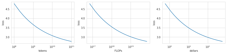
The three plots below shows predictions of the Chinchilla model for \(N_\text{gpt2-sm} = 117 \cdot 10^6\). The firsts two plots show loss as a function of \(D\) and \(C = 6N_\text{gpt2-sm}D\). Intuitively, they show the shape of train loss predicted by the Chinchilla model. The last plot gives a very rough estimate of a price of a training run assuming a 1.2e17 FLOP/dollar from Ajeya Cotra’s report (Appendix).
Compute-optimal dataset size
The Chinchilla paper focuses on compute-optimal models: optimal \((N, D)\) for a fixed \(D\). I’m interested in an inverse problem: what’s an optimal dataset size \(D\) for a model size \(N\). Equivalently, what’s an optimal compute budget \(C\) for a model of size \(N\). There are two intuitive framings of this question:
- When should I stop training? What’s the number of tokens \(D\) such that after \(D\) subsequent decreases in my loss (\(L(N, D+1), L(N, D+2), \dots)\) are small enough that I’d be better off spending my \(6N(D+1)\) FLOPs training a bigger model on fewer tokens.
- How long should I keep training? What’s the number of tokens \(D\) that I need to reach to justify training a model with as many as \(N\) parameters (as opposed to a training a smaller model on more tokens)?
Therefore, a dataset size \(D\) is compute-optimal for model size \(N\) if \((N, D)\) is compute-optimal: every other allocation of \(6ND\) FLOPs results in a worse loss:
\[L(N-1, \frac{N}{N-1}D) > L(N, D) < L(N+1, \frac{N}{N+1}D).\]Compute-optimal dataset for gpt2-small
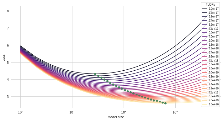
First, we can plot IsoFLOP curves for a range of compute budgets \(10^{16} < C < 10^{20}\). An IsoFLOP curve for budget \(C\) shows loss as a function of \(N\), i.e. \(L(N, \frac{C}{6N})\).

Second, we can find a minimum of each IsoFLOP with respect to \(N\). Each such minimum (marked by a green dot) is a compute-optimal model \((N, D)\) for a given budget \(C\).
Finally, we can look for a compute-optimal model \((N, D)\) with \(N\) closest to \(N_\text{gpt2-sm} = 117 \cdot 10^6\).
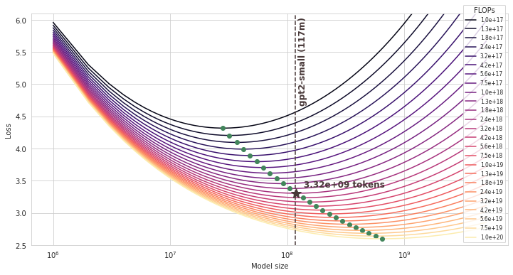
The compute-optimal dataset size turns out to be 3.32B tokens (and the corresponding compute budget is 2.37E+18 FLOPs).
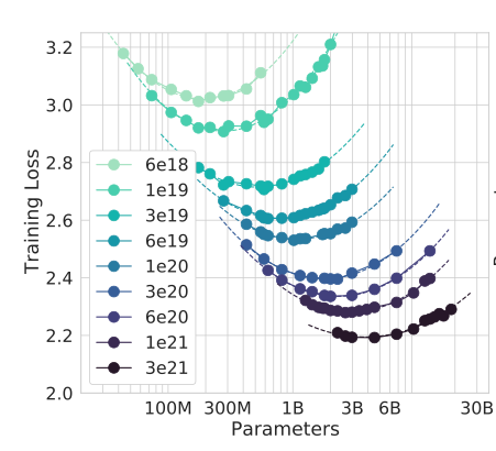
This seems to match results from the Chinchilla paper:
 |
 |
Postscriptum
How much does it cost?
Less than $100 on the cloud. Based on my recent experiments, with two A100 (80gb) GPUs, it takes around 16h to train gpt2-small on 3.3B tokens.
You’d pay $80 for 4xA100 (40gb) on Lambda Labs or around $45 on GCP, in a good region.
How many parameters does gpt2-small have?
While the GPT2 paper says gpt2-small has 117m parameters, the Hugginface implementation actually has 127m:
from transformers import AutoModel
gpt2_small = AutoModel.from_pretrained('gpt2')
gpt2_small.num_parameters()
Not counting embeddings (gpt2_small.num_parameters(exclude_embeddings=True)), it’s 85m which is also quite off. I’m not sure what’s going on here. The difference doesn’t seem to matter much.
What are good hyperparameters?
I found it useful to look at config files of two well-documented open source projects training gpt2-small-sized models: codeparrot and mistral. A Bloom paper called What Language Model to Train if You Have One Million GPU Hours? and the Gopher paper also report some results with gpt2-small-sized models.
Overall, I’d use a linear or cosine learning rate schedule (with warmup_ratio=0.01) and do a sweep over batch sizes and learning rates. For instance, codeparrot-small used learning rate 5e-4 and batch size 192 (197k tokens) while mistral used learning rate 6e-4 and batch size 512 (524k tokens). Similarly, the Gopher paper reports their learning rate and batch size for 117m model to be 6e-4 and 125 (0.25m tokens; note they have context window 2048).
Further reading
- chinchilla’s wild implications offers a great discussion of the Chinchilla scaling law and how it informs the future of language model research
The code I used for the plots is available here