Interpreting uncertainty in Bayesian linear regression

While vanilla linear regression predicts a maximum likelihood estimate of the target variable, Bayesian linear regression predicts a whole distribution over the target variable, offering a natural measure of prediction uncertainty. In this blog post, I demonstrate how to break down this uncertainty measure into two contributing factors: aleatoric uncertainty and epistemic uncertainty. We will dive deeper into the Bayesian framework for doing machine learning and inspect closed-form solutions for training and doing inference with Bayesian linear regression. I will then go on to discuss practical uses of uncertainty estimation: deciding when to stop gathering data, active learning and outlier detection as well as improving model performance by predicting only on a subset of the data.

Bayesian linear regression

Vanilla linear regresion predicts the target value \(y\) based on trained weights \(\mathbf{w}\) and input features \(\mathbf{x}\). Bayesian linear regression predicts the distribution over target value \(y\) by mariginalizing over the distribution over weights \(\mathbf{w}\). Both training and prediction can described in terms of inferring \(y\), which decomposes into two inference problems: inferring \(y\) based on parameters \(\mathbf{w}\) and features \(\mathbf{x}\) (prediction) and inferring weights based on training data (\(\mathbf{X_{train}}, \mathbf{y_{train}}\)) (training).

The distribution over targets \(p(y \vert \mathbf{x}, \mathbf{w})\) is known as the predictive distribution and can be obtained by marginalization over \(\mathbf{w}\). Intuitively, we take the average of predictions of infinitely many models – that’s the essence of the Bayesian approach to machine learning.

Here \(\mathbf{X_{train}}\) and \(\mathbf{y_{train}}\) constitute our training set and \(\alpha\) and \(\beta\) are two hyperparameters. Both of the distributions of the right-hand side have closed-form and there is also a closed-form solution for the predictive distribution. Let’s take a look at those.

Conditional distribution over targets

The distribution over targets conditioned on weights and features is simply a Gaussian with mean determined by a dot product of weights and features (as in vanilla linear regression) and fixed variance determined by a precision parameter \(\beta\).

Parameter distribution

The parameter distribution is also assumed to be a Gaussian governed by mean \(\mathbf{m}_N\) and covariance \(\mathbf{S}_N\).

The parameters \(\mathbf{m}_N\) and \(\mathbf{S}_N\) of the posterior parameter distribution are given by

and

where \(\alpha\) is a parameter governing the precision of a prior parameter distribution \(p(\mathbf{w})\).

Predictive distribution

The predictive distribution is the actual output of our model: for a given \(\mathbf{x}\) it predicts a probability distribution over \(y\), the target variable. Because both the distribution over parameters and the conditional distribution over targets are Gaussians, the predictive distribution is a convolution of these two and also Gaussian, taking the following form:

The mean of the predictive distribution is given by a dot product of the mean of the distribution over weights \(\mathbf{m}_N\) and features \(\mathbf{x}\). Intuitively, we’re just doing vanilla linear regression using the average weights and ignoring the variance of the distribution over weights for now. It is accounted for separately in the variance of the predictive distribution:

The variance of the predictive distribution, dependent on features \(\mathbf{x}\), gives rise to a natural measure of prediction uncertainty: how sure is the model that the predicted value (\(\mathbf{m}_N^\text{T}\mathbf{x}\)) is the correct one for \(\mathbf{x}\). This uncertainty can be further decomposed into aleatoric uncertainty and epistemic uncertainty.

Aleatoric uncertainty represents the noise inherent in the data and is just the variance of the conditional distribution over targets, \(\beta^{-1}\). Since the optimal value of \(\beta^{-1}\) is — as we will see — just the variance of \(p(y \vert \mathbf{x})\), it will converge to the variance of the training set.

Epistemic uncertainty reflects the uncertainty associated with the parameters \(\mathbf{w}\). In principle, it could be reduced by moving the parameter distribution towards a better region given more training examples (\(\mathbf{X_{train}}\) and \(\mathbf{y_{train}}\)).

Can this decomposition be used in practice? I will now proceed to discuss three applications of uncertainty estimation in the context of Bayesian linear regression: a stopping criterion for data collection, active learning and selecting only a subset of the data to predict targets for.

What is uncertainty for?

Bayesian linear regression in scikit-learn

Scikit-learn provided a nice implementation of Bayesian linear regression as BayesianRidge, with fit and predict implemeted using the closed-form solutions laid down above. It also automatically takes scare of hyperparameters \(\alpha\) and \(\beta\), setting them to values maximizing model evidence \(p(\mathbf{y_{train}} \vert \mathbf{X_{train}}, \alpha, \beta)\).

Just for the sake of experiments, I will override predict to access what scikit-learn abstracts away from: my implementation will return aleatoric and epistemic uncertainties rather than just the square root of their sum – the standard deviation of the predictive distribution.

class ModifiedBayesianRidge(BayesianRidge):

    def predict(self, X):
        y_mean = self._decision_function(X)
        if  self.normalize:
            X = (X - self.X_offset_) / self.X_scale_
        aleatoric = 1. / self.alpha_
        epistemic = (np.dot(X, self.sigma_) * X).sum(axis=1)
        return y_mean, aleatoric, epistemic

Note that while I loosely followed the notation in Bishop’s Pattern Recognition and Machine Learning, scikit-learn follows a different convention. self.alpha_ corresponds to \(\beta\) while self.sigma_ corresponds to \(\mathbf{S}_{N}\).

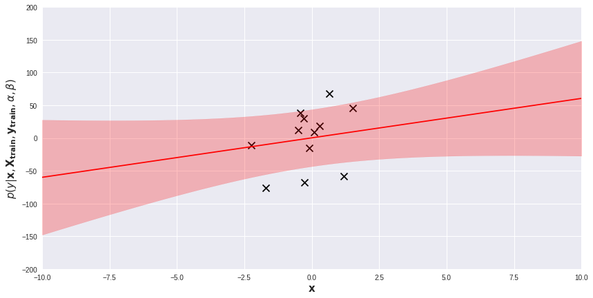
We will experiment with ModifiedBayesianRidge on several toy one-dimensional regression problems. Belove, on a scatter plot visualizing the dataset, I added the posterior predictive distribution of a fitted model. The red line is the average of the predictive distribution for each \(\mathbf{x}\), while the light-red band represents the area within 1 standard deviation (i.e. \(\sqrt{\beta^{-1} + \mathbf{x}^\text{T} \mathbf{S}_N\mathbf{x}}\)) from the mean. Prediction for each data point \(\mathbf{x}\) comes with its own measure of uncertainty. Regions far from training examples are obviously more uncertain for the model. We can exploit these prediction uncertainties in several ways.

When to stop gathering data?

Acquiring more training data is usually the best thing you can do to improve model performance. However, gathering and labeling data is usually costly and offers diminishing returns: there more data you have, the smaller improvements new data bring about. It is hard to predict in advance the value of a new batch of data or to develop a stopping criterion for data gathering/labeling. One way is to plot your performance metric (for instance, test set mean squared error) against training set size and look for a trend. It requires, however, multiple evaluations on a held-out test set, ideally a different one than those used for hyperparameter tuning and final evaluation. In small data problems, we may not want to do that.

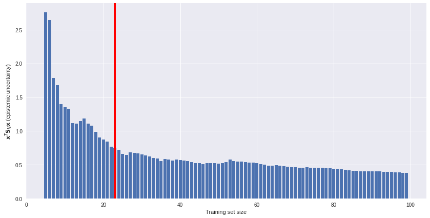
Uncertainty estimates offer an unsupervised solution. We can plot model uncertainty (on an unlabeled subset) against training set size and see how fast (or slow) epistemic uncertainty is reduced as more data is available. An example of such a plot is below. If data gathering is costly, we might decide to stop gathering more data somewhere around the red line. More data offers diminishing returns.

Active learning and outlier detection

Some data points \(\mathbf{x}\) are more confusing for the model than others. We can identify the most confusing data points in terms of epistemic uncertainty and exploit it in two ways: either focusing on the most confusing data when labeling more data or removing the most confusing data points from the training set.

The first strategy is known as active learning. Here we select the new data for labeling based on prediction uncertainties of a model trained on existing data. We will usually want to focus on the data the model is most uncertain about. A complementary approach is outlier detection. Here we assume that the datapoints model is most uncertain about are outliers, artifacts generated by noise in the data generating process. We might decide to remove them from the training set altogether and retrain the model.

Which approach is the best heavily depends on multiple circumstances such as data quality, dataset size and end user’s preferences. Bayesian linear regression is relatively robust against noise in the data and outliers should not be much of a problem for it, but we might want to use Bayesian linear regression just to sanitize the dataset before training a more powerful model, such as a deep neural net. It is also useful to take a look at the ratio between aleatoric and epistemic uncertainty to decide whether uncertainty stems from noise or real-but-not-yet-learned patterns in the data.

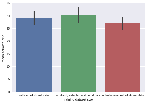
Below I illustrate active learning with a simple experiment. We first train a model on 50 data points and then, based on its uncertainty, select 10 out of 100 data additional data points for labeling. I compare this active learning scheme with a baseline (randomly selecting 10 out of 100 data points for labeling) in terms of mean square error. In the active learning case, it is slightly lower, meaning our carefully selected additional data points reduce the mean squared error better than randomly sampled ones. The effect is small, but sometimes makes a difference.

Doing inference on a subset of the data

We might also do outlier detecion at test time or during production use of a model. In some applications (e.g. in healthcare), the cost of making a wrong prediction is frequently higher than the cost of making no prediction. When the model is uncertain, the right thing to do may be to pass the hardest cases over to a human expert. This approach is sometimes called the reject option.¹

For the sake of illustration, I trained a model on 10 data points and computed test set mean squared error on either the whole test set (10 data points), or 5 data points in the test set the model is most certain about.

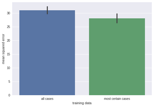
We can obtain slightly smaller error when refraining from prediction on half of the dataset. Is it worth it? Again, it heavily depends on your use case.

Conclusions

The goal of this blog post was to present the mathematics underlying Bayesian linear regression, derive the equations for aleatoric and epistemic uncertainty and discuss the difference between these two, and finally, show three practical applications for uncertainty in data science practice. The notebook with code for all the discussed experiments and presented plots is available on GitHub.

A version of this blog post was originally published on Sigmoidal blog.