Helmholtz machines and variational autoencoders

Helmholtz machines are the predecessors of variational autoencoders (VAEs). They were first proposed by Dayan et al. in 1995 as a probabilistic model of pattern recognition in human visual cortex. In this blog post, I discuss a toy PyTorch implementation of Helmholtz machine and an algorithm proposed to train it — the wake-sleep algorithm. Then, I contrast both with VAEs trained with backpropagation using the reparametrisation trick.

Helmholtz machine objective

A Helmholtz machine learns a generative distribution \(p(x, z)\) over patterns \(x\) and latents \(z\) that minimises the generative free energy or negative model evidence for a pattern \(x\):

This loss is upper bounded by the variational free energy which involves an other distribution, the recognition distribution \(q\):

Alternatively, variational free energy is the generative free energy plus the KL between \(q\) and \(p\).

The wake-sleep algorithm alternates between minimising \(F^p_q(x)\) with respect to the parameters of \(p\) and \(q\).

Wake phase

In the wake phase, minimising \(F^q_p(x)\) with respect to \(p\) a pattern \(x\) from the true distribution \(p^*(x)\) boils down to minimising \(\mathbb{E}_{q(z\vert x)} [-\log p(x,z)]\). Concretely, we sample a latent state \(z\) from \(q(z\vert x)\), and minimise \(-\log p(x, z)\) decomposed as \(-\log p(x\vert z) -\log p(x)\).

Sleep phase

In the sleep phase, we minimise \(F^q_p(x)\) with respect to \(q\). To that end, use an approximation taking the second form of \(F^R_G(d)\) and reversing the KL:

Minimising this quantity boils down to minimising \(\mathbb{E}_{p(x,z)} [-\log q(z \vert x)]\).

Wake-sleep algorithm as expectation maximisation

There is an elegant symmetry between these two phases that’s worth reiterating:

• In wake phase, we minimise \(\mathbb{E}_{q(z\vert x)} [-\log p(x,z)]\) w.r.t. \(p\),
• In sleep phase, we minimise \(\mathbb{E}_{p(x,z)} [-\log q(z\vert x)]\) w.r.t. \(q\).

Crucially, we always optimise the distribution that we’re not sampling from. That allows for propagating the gradients through samples without reparametrisation: generally, \(\nabla_\theta \mathbb{E}_{p(x)} f(x) = \mathbb{E}_{p(x)} \nabla_\theta f(x)\) if \(p\) is not parametrised by \(\theta\). Indeed, as we’ll see wake-sleep is a way of training latent variable models before the reparametrisation trick was invented/popularised by Kingma and Welling and Rezende et al. in 2014. It can also be seen as an EM algorithm alternating between optimising \(q\) (the E-step) and \(p\) (the M-step).

Training a Helmholtz machine for MNIST generation

A Helmholtz machine can be implemented in a few lines of PyTorch. The below implementation differs from the the original algorithm of Dayan et al. in one respect: there is a single latent variable \(z\) parametrised by a two-layer feedforward neural network while Dayan et al. treated the activations of both layers as latent variables. Moreover, Dayan et al. optimised \(p\) and \(q\) using a local learning rule, the delta rule, while I utilise backpropagation to train both layers end-to-end (but separately for the encoder and the decoder). This is to be as close to the standard VAE setup as possible.

class HelmholtzMachine(torch.nn.Module):

    def __init__(self, input_size, latent_size, batch_size):
        super().__init__()
        self.latent_size = latent_size
        self.batch_size = batch_size
        self.encoder = torch.nn.Sequential(
            torch.nn.Linear(input_size, latent_size*2),
            torch.nn.ReLU(),
            torch.nn.Linear(latent_size*2, latent_size),
            torch.nn.Sigmoid(),
        )
        self.encoder_optimizer = torch.optim.SGD(
            params=self.encoder.parameters(), 
            lr=1e-3
            )
        self.decoder = torch.nn.Sequential(
            torch.nn.Linear(latent_size, latent_size*2),
            torch.nn.ReLU(),
            torch.nn.Linear(latent_size*2, input_size),
            torch.nn.Sigmoid(),
        )
        self.latent_prior = torch.nn.Parameter(torch.zeros(self.latent_size)/2)
        self.decoder_optimizer = torch.optim.SGD(
            params=list(self.decoder.parameters()) + [self.latent_prior], 
            lr=1e-3
        )

    def wake(self, input):
        with torch.no_grad():
            latent_state = torch.bernoulli(self.encoder(input))
        reconstruction = self.decoder(latent_state)
        reconstruction_loss = binary_cross_entropy(reconstruction, input, reduction='sum')
        regularisation_penalty = binary_cross_entropy(
            torch.sigmoid(self.latent_prior).repeat(self.batch_size, 1), 
            latent_state, 
            reduction='sum'
        )
        loss = reconstruction_loss + regularisation_penalty
        loss.backward()
        self.decoder_optimizer.step()
        self.decoder_optimizer.zero_grad()

    def sleep(self):
        with torch.no_grad():
            sampled_latent_state = torch.bernoulli(
                torch.sigmoid(self.latent_prior).repeat(self.batch_size, 1)
            )
            generated_image = self.decoder(sampled_latent_state)
        inferred_latent_state = self.encoder(generated_image)
        loss = binary_cross_entropy(
            inferred_latent_state, 
            sampled_latent_state, 
            reduction='sum'
        )
        loss.backward()
        self.encoder_optimizer.step()
        self.encoder_optimizer.zero_grad()
    
    def generate(self, n):
        with torch.no_grad():
            sampled_latent_state = torch.bernoulli(
                torch.sigmoid(self.latent_prior).repeat(n, 1)
            )
            return self.decoder(sampled_latent_state)

The torch.no_grad context manager hopefully makes it clear which network is being optimised during which phase. The training loop involves alternating between the two phases.

dataset = MNIST('.', train=True, transform=ToTensor(), download=True)
loader = DataLoader(dataset=dataset, batch_size=128, drop_last=True)
machine = HelmholtzMachine(input_size=784, latent_size=10, batch_size=128)
for _ in range(10):
    for batch, _ in loader:
        machine.wake(batch.view(128, 784))
        machine.sleep()

I wasn’t able to get Helmholtz machines to produce high-quality reconstructions: they tend to capture at most several modes of the distribution but not all of them.

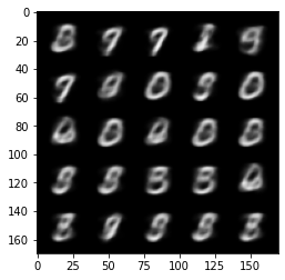Images generated from \(p(x \vert z)\) when sampling \(z \sim \mathcal{N}(0, 1)\)

Variational autoencoders

Variational autoencoders are based on a third formulation of the variational free energy objective:

which is obtained by decomposing the log joint \(\log p(x,z) = \log(x \vert z) -\log p(z)\) and using \(-\log p(z)\) to complete the KL. Consider a simplified implementation of VAE below just for comparison.

class VAE(torch.nn.Module):

    def __init__(self, input_size, latent_size):
        super().__init__()
        self.latent_size = latent_size
        self.encoder = torch.nn.Sequential(
            torch.nn.Linear(input_size, latent_size*2),
            torch.nn.Linear(latent_size*2, latent_size*2),

            torch.nn.ReLU(),
        )
        self.encoder_mu = torch.nn.Linear(latent_size*2, latent_size)
        self.encoder_log_var = torch.nn.Linear(latent_size*2, latent_size)
        self.decoder = torch.nn.Sequential(
            torch.nn.Linear(latent_size, latent_size*2),
            torch.nn.ReLU(),
            torch.nn.Linear(latent_size*2, input_size),
            torch.nn.Sigmoid(),
        )

    def forward(self, input):
        activations = self.encoder(input)
        mu = self.encoder_mu(activations)
        log_var = self.encoder_log_var(activations)
        std = torch.exp(0.5 * log_var)
        latent_state = mu + torch.randn_like(std) * std
        reconstruction = self.decoder(latent_state)
        reconstruction_loss = binary_cross_entropy(
            reconstruction, 
            input, 
            reduction='sum'
        )    
        kld_loss = -torch.sum(1 + log_var - mu**2 - torch.exp(log_var))/2
        return reconstruction_loss + kld_loss

    def generate(self, n):
        with torch.no_grad():
            sampled_latent_state = torch.randn(n, self.latent_size)
            return self.decoder(sampled_latent_state)

The two phases of learning are merged into one: we simultaneously minimise the reconstruction loss part of the loss \(\mathbb{E}_{q(z \vert x)} [-\log p(x \vert z)]\) with respect to both \(p\) and \(q\). A few steps were needed to make that possible:

1. First, we assume our latent state \(z\) to be a Gaussian random variable as opposed to a Bernoulli random variable.
2. This makes it possible to apply a reparametrisation \(z = \mu + \sigma \epsilon\), where \(\epsilon \sim \mathcal{N}(0, 1)\) and \(\mu\) and \(\sigma\) are parameters predicted by the encoder network.
3. This allows for reformulating the reconstruction loss as \(\mathbb{E}_{\epsilon \sim \mathcal{N}(0, 1)} [-\log p(x \vert \mu + \sigma \epsilon)]\), which is differentiable with respect to both \(p\) and \(q\).

Why start with Bernoulli latents in the first place? The motivation for Dayan et al. is clearly biological plausibility: a sample from a Bernoulli distribution represents spikes of biological neurons. This is particularly interesting in conjunction with the fact that the alternating training scheme allows for purely local learning rules: during sleep phase, the activations of the decoder are treated as ground truth values when optimising the encoder using delta rules. Thus, one can get rid of backprop in favour of a biologically plausible local computations. (This is not how my toy implementation works, though: I used backprop within the encoder and the decoder to highlight similarities with VAEs)

On the other hand, training \(p\) and \(q\) end-to-end in VAEs is very powerful. It produces much better images and in general allows for learning much more complex, high-dimensional distributions.

Further reading

The original paper for Helmholtz machines is somewhat cryptic and Kevin Kirby’s tutorial paper is a better starting point. Moreover, Shakir Mohamed has a great blog post on reparametrisation.

This blog post benefited greatly from discussions with Chris Buckley. An accompanying notebook is available on GitHub.