EM for Gaussian mixtures using einsum

The goal of this blogpost is to present a concise implementation of the Gaussian Mixture Model (GMM) using einsum notation. Along the way, I will also describe the expectation-maximization (EM) algorithm.

Einsum

Einstein notation is a particular convention of writing tensor operations that is implemented in NumPy, PyTorch and other deep learning frameworks. Its essence lies in indicating summations implicitly: the summation is over indices that are skipped or occur repeatedly. For instance, a batched bilinear transformation \(d = aBc\), for \(a \in \mathbb{R}^{B \times I}, B \in \mathbb{R}^{B \times I \times J}, c \in \mathbb{E}^{B \times J}\), can be wrriten as \(d_b = a_i B_{ij} c_j\) or np.einsum('bi,bij,bj->b', a, B, c). As I will show below, it is particularly useful when dealing with mixtures or multivariate Gaussians, which are effectively 3-dimensional tensors.

Tim Rocktäschel has a nice introductory post on einsum in the context of deep learning.

Gaussian mixtures

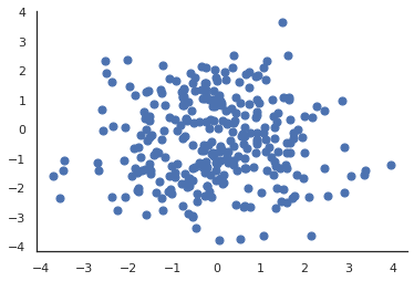
Let’s assume we have a dataset \(X\) of \(N\) data points in an \(D\)-dimensional space. Here \(D=2\) and \(N=100\).

def create_dataset():
    x1 = np.random.normal(size=(100, 2)) + np.array([-1, -1])
    x2 = np.random.normal(size=(100, 2)) + np.array([1, -1])
    x3 = np.random.normal(size=(100, 2)) + np.array([0, 1])
    return np.vstack((x1, x2, x3))
X = create_dataset()
plt.scatter(X[:, 0], X[:, 1], cmap='gist_rainbow', s=50)
sns.despine()

The dataset \(X \in \mathbb{R}^D\) for our motivating example

We would like to discover clusters in the data and assign each point \(x_n \in X\) with a categorical probability distribution over \(K\) clusters. To that end, we will try to model the dataset as a mixture of \(K\) Gaussians.

Gaussian mixtures can be posed as latent variable models of the following form:

where the first product is over data points and the second over mixture components. \(z_{nk}\) is a latent variable determining whether \(n\)-th data point belongs to \(k\)-th mixture components and the parameters are \(\theta = \{\pi_k, \mu_k, \Sigma_k\}_k\).

Will will implement our GMM as a class GaussianMixture with a scikit-learn-like API:

class GaussianMixture:

    def __init__(self, num_components, input_size, max_iter=10):
        self.num_components = num_components
        self.input_size = input_size
        self.max_iter = max_iter

        # Parameters
        self.pi = np.ones((self.num_components))/self.num_components
        self.mu = np.random.normal(size=(self.num_components, self.input_size))
        self.sigma = np.tile(np.eye(self.input_size), (self.num_components, 1, 1))

When fitting the model, we are interested in maximising the logarithm of \(p_\theta(X,Z)\):

To make this problem, we instead maximise the following lower bound

where \(q(z \vert x)\) is a variational distribution introduced for convenience: a categorical over \(K\) components. \(\mathcal{L}\) is is known as the ELBo or evidence lower bound as it is always the case that \(\mathcal{L} \leq p_\theta(X)\).

The EM algorithm

EM is an algorithm for maximum likelihood (or maximum a posteriori) estimation of parameters for latent variable models. The algorithm is iterative: we alternate between minimising \(\mathcal{L}(\theta, q)\) with respect to \(\theta\) and updating \(q\) to make the bound tighter, each time fixing one and updating the other. We to that until \(\mathcal{L}\) stops increasing.

def fit(self, X):
    prev_elbo = -np.inf
    for i in range(self.max_iter):
        q = self._expect(X)
        self.pi, self.mu, self.cov = self._maximize(X, q)
        elbo = self.compute_elbo(X, q)
        if np.allclose(elbo, prev_elbo):
            break
        prev_elbo = elbo

E-step

In the E-step, we infer the \(q(z \vert x)\) that inverts \(p_\theta(x \vert z)\) for current \(\theta\) as determined by Bayes’ theorem. For a particular data point \(n\) and a component \(k\), we have:

def _expect(self, X):
    n = X.shape[0]
    c = self.num_components
    d = self.input_size
    pi = self.pi.reshape((1, c))
    X = X.reshape((n, 1, d))
    mu = self.mu.reshape((1, c, d))
    inv_sigma = np.linalg.inv(self.sigma)
    det_sigma = np.linalg.det(self.sigma)
    distance =  np.einsum('ncd,cde,nce->nc', X - mu, inv_sigma, X - mu)
    Z = np.sqrt(det_sigma) * (2 * np.pi) ** (d/2)
    p_x_given_t = np.einsum('nc,c->nc', np.exp(-distance/2), 1/Z)
    q_unnormalized = p_x_given_t * pi
    return q_unnormalized/q_unnormalized.sum(axis=1, keepdims=True)

M-step

In the M-step, we maximise \(\mathcal{L}\) with respect to \(\theta\) given \(q(z \vert x)\) from the E-step. There are closed-form solutions for each of the parameters:

where \(N_k = \sum_{n=1}^N q(z_k \vert x_n)\) can be interpreted as a pseudo-count of data points assigned to component \(k\).

def _maximize(self, X, q):
    n = X.shape[0]
    c = self.num_components
    d = self.input_size
    nk = q.sum(axis=0).reshape((c, 1))
    mu = np.einsum('nd,nc->cd', X, q)/nk
    error = X.reshape((n, 1, d)) - mu.reshape((1, c, d))
    sigma = np.einsum('ncd,nce,nc->cde', error, error, q)/nk.reshape(c, 1, 1)
    pi = (nk/n).reshape((c,))
    return pi, mu, sigma

Computing the ELBo

Finally, a we also need to compute the ELBo which we use as a stopping criterion (although in principle it could also be used as a validation metric or a debugging tool). Recall that the ELBo is just

def compute_elbo(self, X, q):
    n = X.shape[0]
    c = self.num_components
    d = self.input_size
    q += 10e-20
    pi = self.pi.reshape((1, c))
    X = X.reshape((n, 1, d))
    mu = self.mu.reshape((1, c, d))
    inv_sigma = np.linalg.inv(self.sigma)
    logdet_sigma = np.linalg.slogdet(self.sigma)[1].reshape(1, c)
    distance = np.einsum('ncd,cde,nce->nc', X - mu, inv_sigma, X - mu)
    constants = -d/2*np.log(2*np.pi)
    log_p_x_given_t = constants - logdet_sigma/2 - distance.reshape((n, c))/2
    log_pi = np.log(pi).reshape((1, c))
    log_q = np.log(q)
    return ((log_pi + log_p_x_given_t - log_q) * q).sum()

Using the model

Since our latent \(q(z_k \vert z_n)\) is interpretable as cluster assignments, clustering the data boils down to running the E-step with a trained model:

def predict(self, X):
    return self._expect(X)

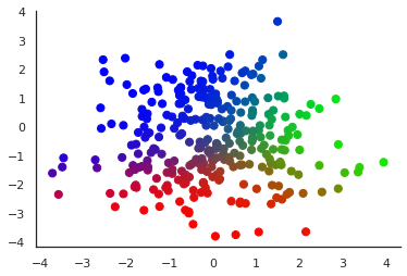
Let us illustrate the obtained components by colour-coding soft cluster assignments:

gmm = GaussianMixture(num_components=3, input_size=2)
gmm.fit(X)
y = gmm.predict(X)
plt.scatter(X[:, 0], X[:, 1], c=y, cmap='gist_rainbow', s=50)
sns.despine()

The dataset \(X\) with each \(x_n\) displayed in a colour obtained from interpreting the vector \(q(z \vert x_n)\) as an RGB triplet: \(z_{n1}\) codes for the value of the red component, \(z_{n2}\) for green and \(z_{n3}\) for blue

EM and the wake-sleep algorithm

There is a non-trivial connection between the EM algorithm and the wake-sleep algorithm I described earlier. The wake step corresponds to the M-step: minimizing the ELBo w.r.t. \(p_\theta\). The sleep step corresponds to the E-step with an important quirk: the input is not an \(x\) sampled from the dataset \(X\), but a synthetic example sampled from \(p(x \vert z)\), where the \(z\) is in turn sampled from a prior \(p(z)\). Moreover, the \(q(z \vert x)\) is an amortised model: it is parametrised by some weights that are should minimise the ELBo across data points.

A notebook accompanying this blog post is available on GitHub. It also contains some tests of my einsum implementation against a simpler one with an explicit for loop over \(K\) components and calls to scipy.stats.multivariate_normal.